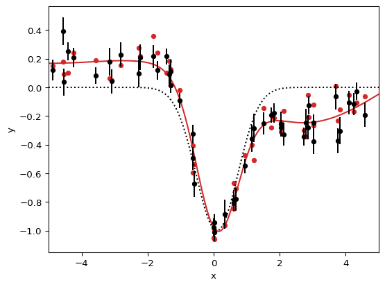
The Gaussian Process Case

Gaussian Process

This notebook is part of a set of examples for teaching Bayesian inference methods and probabilistic programming, using the numpyro library.

Imports
import io
import math

import arviz as az
import jax
import jax.numpy as jnp
import jaxopt
import matplotlib.pyplot as plt
import numpy as np
import numpyro
import numpyro.distributions as dist
import pandas as pd

from jax.typing import ArrayLike
from tinygp import GaussianProcess, kernels
Constants
FIGSIZE = (6.4, 4.8)
TEXTSIZE = 10
RNG Setup
rng_key = jax.random.PRNGKey(1)

In this example, we will reproduce the “model fitting with correlated noise” tutorial from the documentation of the george library, using the tinygp library instead. tinygp is a lightweight library for building Gaussian Process (GP) models, built on top of jax.

Data

Data
csv = """
x,y,y_err
-4.862316,0.119011,0.072891
-4.566759,0.39243,0.09602
-4.526447,0.03616,0.093953
-4.401908,0.252323,0.062631
-4.246188,0.205874,0.0674
-3.562332,0.080907,0.059129
-3.157129,0.178284,0.09509
-3.084805,0.041965,0.085326
-2.812079,0.229085,0.086333
-2.274074,0.096489,0.095004
-2.235357,0.209088,0.088958
-1.831639,0.216567,0.079958
-1.703316,0.119445,0.064556
-1.421827,0.215532,0.05757
-1.35114,0.092736,0.066759
-1.31176,0.112926,0.082878
-1.297492,0.016536,0.053667
-1.027974,-0.09196,0.05275
-0.638266,-0.325933,0.06616
-0.622723,-0.495434,0.079524
-0.578592,-0.673282,0.092695
0.009951,-0.977624,0.064353
0.029668,-1.014229,0.058653
0.030832,-0.9436,0.056701
0.333102,-0.885644,0.099733
0.611962,-0.80845,0.058975
0.614331,-0.783845,0.065877
0.680987,-0.781937,0.078415
0.946248,-0.54763,0.050467
1.153962,-0.356636,0.095032
1.221088,-0.284847,0.098862
1.513781,-0.250288,0.077845
1.748809,-0.194554,0.054239
1.834629,-0.179785,0.06665
2.04261,-0.25717,0.086421
2.045813,-0.282465,0.057122
2.12702,-0.326968,0.077623
2.728266,-0.342656,0.063652
2.799758,-0.24829,0.098725
2.853586,-0.278951,0.083389
2.887301,-0.125747,0.062783
3.018722,-0.245938,0.055416
3.021476,-0.377726,0.088809
3.691274,-0.063975,0.089124
3.759326,-0.37162,0.08808
3.826412,-0.302928,0.09572
4.09316,-0.108121,0.082931
4.248676,-0.117814,0.078418
4.331401,-0.028635,0.060088
4.581394,-0.193597,0.084915
"""

data = pd.read_csv(io.StringIO(csv))
x y y_err
0 -4.862316 0.119011 0.072891
1 -4.566759 0.392430 0.096020
2 -4.526447 0.036160 0.093953
3 -4.401908 0.252323 0.062631
4 -4.246188 0.205874 0.067400
... ... ... ...
45 3.826412 -0.302928 0.095720
46 4.093160 -0.108121 0.082931
47 4.248676 -0.117814 0.078418
48 4.331401 -0.028635 0.060088
49 4.581394 -0.193597 0.084915

50 rows × 3 columns

Given the above \(n=50\) data points \((x_i, y_i)\) with estimated measurement errors \(\varepsilon_i\) (\(i=1\dots n\)), we are going to infer four parameters of interest that describe a single Gaussian feature - an offset \(\overline{y}\), an amplitude \(a\), a location \(\overline{x}\), and a width \(\sigma\):

\[y(x)=\overline{y}+a\,\exp\left(-\frac{1}{2}\frac{(x-\overline{x})^2}{\sigma^2}\right)\]

This feature appears on top of correlated noise that we are going to model using a GP, adding three more parameters to the final parameter vector \(\boldsymbol{\theta}\) - a noise amplitude \(\eta\) and scale \(\tau\), as well as an additional component of uncorrelated noise \(\overline{\varepsilon}\) (“jitter”). The final likelhood function is a multivariate Gaussian distribution:

\[\log p\left(\{y_i\}\right|\{x_i\},\{\varepsilon_i\},\boldsymbol{\theta})=-\frac{1}{2}\mathbf{r}^TK^{-1}\mathbf{r}-\frac{1}{2}\log\det K-\frac{n}{2}\log 2\pi\]

Here, \(\mathbf{r}\) is the residual vector and \(K\) the covariance matrix, with elements:

\[r_{i}=y_i-y(x_i)\]

\[K_{ij}=(\varepsilon_i^2+\overline{\varepsilon}^2)\delta_{ij}+k(x_i,x_j)\]

To model the off-diagonal elements of \(K\), we’ll use a “squared exponential” kernel:

\[k(\Delta x=|x_i-x_j|)=\eta^2\exp\left(-\frac{1}{2}\frac{\Delta x^2}{\tau^2}\right)\]

class Model:
    def __init__(
        self,
        offset: float,
        amplitude: float,
        location: float,
        sigma: float,
        gp_amplitude: float,
        gp_scale: float,
        gp_jitter: float,
    ) -> None:
        # model parameters
        self._offset = offset
        self._amplitude = amplitude
        self._location = location
        self._sigma = sigma
        # noise parameters
        self._gp_amplitude = gp_amplitude
        self._gp_scale = gp_scale
        self._gp_jitter = gp_jitter

    @property
    def params(self) -> dict[str, float]:
        return {
            "offset": self._offset,
            "amplitude": self._amplitude,
            "location": self._location,
            "sigma": self._sigma,
            "gp_amplitude": self._gp_amplitude,
            "gp_scale": self._gp_scale,
            "gp_jitter": self._gp_jitter,
        }

    def __call__(self, x: ArrayLike) -> ArrayLike:
        return self._offset + self._amplitude * jnp.exp(
            -0.5 * ((x - self._location) / self._sigma) ** 2
        )

    def construct(self, x: ArrayLike, y_err: ArrayLike) -> GaussianProcess:
        return GaussianProcess(
            kernel=self._gp_amplitude**2 * kernels.ExpSquared(self._gp_scale),
            X=x,
            diag=y_err**2 + self._gp_jitter**2,
            mean=self,
        )
true_model = Model(
    offset=0.0,
    amplitude=-1.0,
    location=0.1,
    sigma=math.sqrt(0.4),
    gp_amplitude=math.sqrt(0.1),
    gp_scale=3.3,
    gp_jitter=1e-6,
)
x_grid = np.linspace(-5, 5, 500)
Figure
def plot_data(ax=None):
    if ax is None:
        _, ax = plt.subplots(figsize=FIGSIZE)

    data.plot.scatter(x="x", y="y", yerr="y_err", s=20, color="k", zorder=1, ax=ax)
    ax.plot(x_grid, true_model(x_grid), color="k", ls="dotted", zorder=1)

    ax.set_xlim(np.min(x_grid), np.max(x_grid))
    ax.set_xlabel("x")
    ax.set_ylabel("y")
    return ax


def plot_model(rng_key, ax=None):
    ax = plot_data(ax=ax)
    gp = true_model.construct(data.x.values, data.y_err.values)
    _, gp_con = gp.condition(data.y.values, diag=data.y_err.values ** 2)
    ax.scatter(data.x, gp_con.sample(rng_key), s=20, color="C3", zorder=-1)
    _, gp_con = gp.condition(data.y.values, x_grid)
    ax.plot(x_grid, gp_con.mean, color="C3", zorder=-1)
    return ax


rng_key, _rng_key = jax.random.split(rng_key)
plot_model(_rng_key)
plt.show()

Figure 1: The data points (black dots) together with the true feature (dotted line), as well as another sample of data points from the GP that was used to generate the original data points (red dots), and its mean function (red line).

Model

def model(df: pd.DataFrame, x_pred: ArrayLike | None = None) -> None:
    x_meas = numpyro.param("x_meas", df.x.values)
    y_meas = numpyro.param("y_meas", df.y.values)
    y_err = numpyro.param("y_err", df.y_err.values)

    model = Model(
        offset=numpyro.sample("offset", dist.Normal(0, 1)),
        amplitude=numpyro.sample("amplitude", dist.Uniform(-2, 0)),
        location=numpyro.sample("location", dist.Normal(0, 5)),
        sigma=numpyro.sample("sigma", dist.LogUniform(0.1, 1)),
        gp_amplitude=numpyro.sample("gp_amplitude", dist.HalfNormal(1)),
        gp_scale=numpyro.sample("gp_scale", dist.HalfNormal(10)),
        gp_jitter=numpyro.sample("gp_jitter", dist.HalfNormal(1)),
    )

    gp = model.construct(x_meas, y_err)

    with numpyro.plate("data", len(y_meas)):
        numpyro.sample("y_obs", gp.numpyro_dist(), obs=y_meas)

    if x_pred is not None:
        numpyro.deterministic("y_pred", model(x_pred))
sampler = numpyro.infer.MCMC(
    sampler=numpyro.infer.NUTS(
        model,
        init_strategy=numpyro.infer.init_to_value(values=true_model.params),
    ),
    num_warmup=2000,
    num_samples=4000,
    num_chains=4,
    progress_bar=False,
)
rng_key, _rng_key = jax.random.split(rng_key)
sampler.run(_rng_key, data)
inf_data = az.from_numpyro(sampler)
Figure
def plot_trace(ax=None):
    return az.plot_trace(data=inf_data, figsize=(FIGSIZE[0], 7 * 2), axes=ax)


plot_trace()
plt.tight_layout()
plt.show()

Figure 2: The MCMC trace plot.
Table
az.summary(inf_data, kind="all")
mean sd hdi_3% hdi_97% mcse_mean mcse_sd ess_bulk ess_tail r_hat
amplitude -1.052 0.013 -1.077 -1.027 0.000 0.000 10093.0 12263.0 1.0
gp_amplitude 0.177 0.010 0.158 0.195 0.000 0.000 13810.0 12536.0 1.0
gp_jitter 0.028 0.003 0.022 0.034 0.000 0.000 15620.0 9088.0 1.0
gp_scale 2.161 0.089 1.996 2.328 0.001 0.001 10119.0 10966.0 1.0
location 0.089 0.005 0.079 0.098 0.000 0.000 19961.0 12930.0 1.0
offset 0.047 0.016 0.015 0.076 0.000 0.000 17631.0 12181.0 1.0
sigma 0.650 0.006 0.638 0.662 0.000 0.000 10840.0 12148.0 1.0

Results

Figure
def plot_pair(ax=None):
    return az.plot_pair(
       data=inf_data,
       figsize=FIGSIZE,
       var_names=["~gp_"],
       filter_vars="regex",
       kind=["hexbin", "kde"],
       hexbin_kwargs={"cmap": "YlGn"},
       marginals=True,
       marginal_kwargs={"color": "k"},
       reference_values=true_model.params,
       reference_values_kwargs={"color": "red"},
       textsize=TEXTSIZE,
       ax=ax,
    )


plot_pair()
plt.show()

Figure 3: The joint posterior distribution of the parameters of interest, shown together with the true values.

Let’s also find the maximum-likelihood solution:

def loss_factory(df):
    @jax.jit
    def loss(params):
        gp = Model(**params).construct(df.x.values, df.y_err.values)
        return -gp.log_probability(df.y.values)

    return loss


fit = jaxopt.LBFGS(fun=loss_factory(data)).run(
    jax.tree_util.tree_map(jnp.asarray, true_model.params)
)
predictive = numpyro.infer.Predictive(model, sampler.get_samples())

rng_key, _rng_key = jax.random.split(rng_key)
pred_data = az.from_numpyro(
    posterior_predictive=predictive(_rng_key, df=data, x_pred=x_grid)
)
Figure
def plot_pred(ax=None):
    ax = plot_data(ax=ax)

    samples = az.extract(pred_data, group="posterior_predictive", var_names=["y_pred"])
    percentiles = np.percentile(samples, [3, 97], axis=1)
    ax.fill_between(x_grid, *percentiles, color="k", alpha=0.25, zorder=-1)

    model = Model(**fit.params)
    gp = model.construct(data.x.values, data.y_err.values)
    _, gp_con = gp.condition(data.y.values, x_grid)
    std = np.sqrt(gp_con.variance)
    ax.plot(x_grid, model(x_grid), color="k", zorder=-1)
    ax.plot(x_grid, gp_con.mean, color="C1", zorder=-2)
    y1, y2 = gp_con.mean - std, gp_con.mean + std
    ax.fill_between(x_grid, y1, y2, color="C1", alpha=0.5, zorder=-2)

    return ax


plot_pred()
plt.show()

Figure 4: The maximum-likelihood model (black line) and the corresponding GP mean function (orange line), shown together with the true feature (dotted line) and the data points (black dots) as in Figure 1.

Resources

Watermark

Python implementation: CPython
Python version       : 3.11.13
IPython version      : 9.7.0

pandas    : 2.3.3
numpy     : 2.3.4
jaxopt    : 0.8.5
arviz     : 0.22.0
jax       : 0.8.0
numpyro   : 0.19.0
matplotlib: 3.10.7
tinygp    : 0.3.0