This notebook is part of a set of examples for teaching Bayesian inference methods and probabilistic programming, using the numpyro library.
Imports
import ioimport arviz as azimport jaximport jax.numpy as jnpimport matplotlib.pyplot as pltimport numpy as npimport numpyroimport numpyro.distributions as distimport numpyro.handlersimport numpyro.inferimport pandas as pdimport scipy.statsfrom arviz.labels import MapLabellerfrom IPython.display import displayfrom numpyro.infer.reparam import LocScaleReparam
Constants
= (6.4 , 4.8 )= 10 = {"marker" : "o" , "ls" : "none" , "lw" : 2 , "capsize" : 4 }= {"c" : "gray" , "ls" : "dotted" }= MapLabeller({"sigma" : r"$\sigma$ (km/s)" , "v0" : r"$v_0$ (km/s)" })
RNG Setup
= jax.random.PRNGKey(1 )
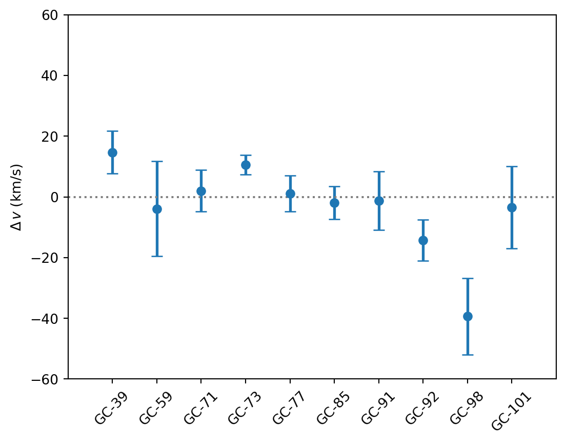
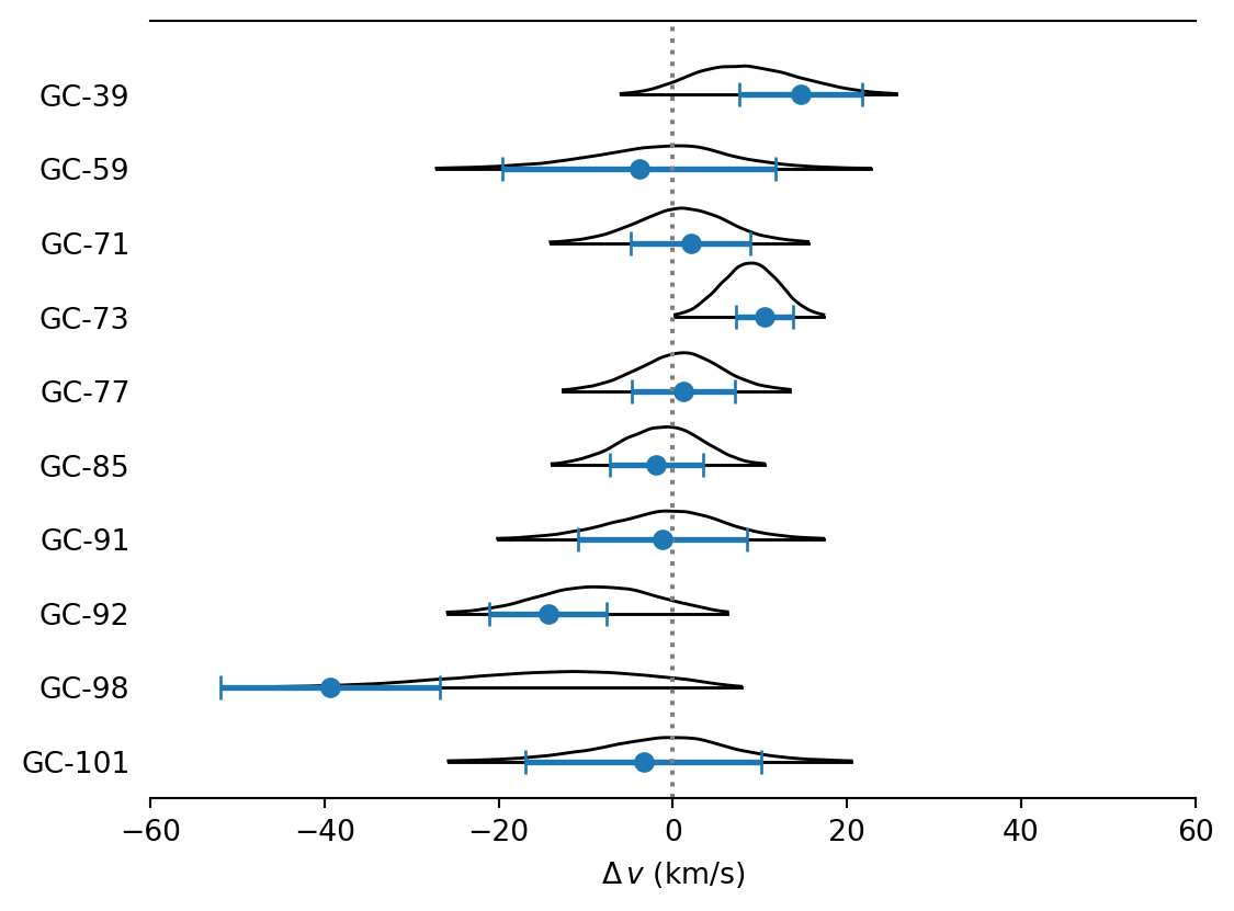
The data consists of radial (line-of-sight) velocities measured for ten globular-cluster-like objects in the ultra-diffuse galaxy NGC1052–DF2. In this example, we will estimate a velocity dispersion from these measurements, taking into account the given measurement uncertainties. From this velocity dispersion, it is possible to estimate the total mass of the galaxy halo, and thus its dark matter fraction (by comparison with its independently estimated stellar mass).
Data
Data
= """ name,v,v_err GC-39,14.728960068829865,7.046858966028704 GC-59,-3.8926505316836715,15.641403662859219 GC-71,2.0484049489377583,6.883925810744802 GC-73,10.576494786228665,3.2586631056780107 GC-77,1.1716309895635035,5.906326879041401 GC-85,-1.9077877208626857,5.3767941243687225 GC-91,-1.2121402228903977,9.69434349499684 GC-92,-14.32028284765569,6.761636322084257 GC-98,-39.335899515592,12.586586245681328 GC-101,-3.3753512069869345,13.523451888563756 """ = pd.read_csv(io.StringIO(csv))
Figure
def plot_data(ax= None ):if ax is None := plt.subplots(figsize= FIGSIZE)= data.index, y= data["v" ], yerr= data["v_err" ], ** MARKER_STYLE)0 , ** INDICATOR_STYLE)= data["name" ], rotation= 45 )r"$\Delta\,v$ (km/s)" )- 1 , 10 )- 60 , 60 )return ax
0
GC-39
14.728960
7.046859
1
GC-59
-3.892651
15.641404
2
GC-71
2.048405
6.883926
3
GC-73
10.576495
3.258663
4
GC-77
1.171631
5.906327
5
GC-85
-1.907788
5.376794
6
GC-91
-1.212140
9.694343
7
GC-92
-14.320283
6.761636
8
GC-98
-39.335900
12.586586
9
GC-101
-3.375351
13.523452
Model
def model(df):= numpyro.param("v_meas" , df["v" ].values)= numpyro.param("v_err" , df["v_err" ].values)= numpyro.sample("v0" , dist.Uniform(- 50 , 50 ))= jnp.exp(numpyro.sample("log_sigma" , dist.Uniform(np.log(0.5 ), np.log(50 ))))with numpyro.plate("data" , len (df)):with numpyro.handlers.reparam(config= {"v" : LocScaleReparam(0 )}):= numpyro.sample("v" , dist.Normal(v0, sigma))"v_obs" , dist.Normal(v, v_err), obs= v_meas)
Figure
= model,= (data,),= True ,= True ,
Sampling
= numpyro.infer.MCMC(= numpyro.infer.NUTS(model),= 2000 ,= 10000 ,= 4 ,= False ,
= jax.random.split(rng_key)
= az.from_numpyro(sampler)"sigma" ] = np.exp(inf_data.posterior["log_sigma" ])
Figure
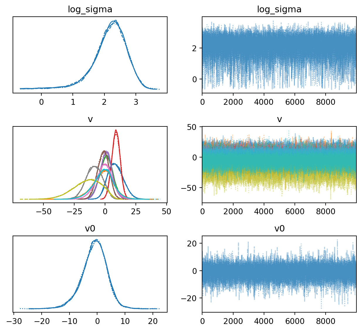
def plot_trace(ax= None ):return az.plot_trace(= inf_data,= (FIGSIZE[0 ], 3 * 2 ),= ["~v_decentered" , "~sigma" ],= ax,
Table
= "all" , var_names= ["~v_decentered" , "~sigma" ])
log_sigma
2.170
0.572
1.157
3.197
0.006
0.008
9047.0
10129.0
1.0
v[0]
8.650
6.255
-2.701
20.567
0.035
0.028
30636.0
30047.0
1.0
v[1]
-1.606
8.924
-19.492
14.748
0.048
0.050
35865.0
29076.0
1.0
v[2]
1.125
5.550
-9.259
11.757
0.023
0.027
59429.0
32620.0
1.0
v[3]
8.884
3.354
2.590
15.241
0.020
0.017
29404.0
22218.0
1.0
v[4]
0.739
4.978
-8.737
10.055
0.020
0.023
59184.0
33754.0
1.0
v[5]
-1.413
4.705
-10.320
7.317
0.021
0.022
49588.0
33222.0
1.0
v[6]
-0.883
7.008
-14.509
11.999
0.032
0.036
48949.0
33351.0
1.0
v[7]
-8.952
6.517
-20.825
3.281
0.042
0.030
23197.0
17708.0
1.0
v[8]
-14.822
11.393
-35.804
4.959
0.092
0.052
14216.0
17665.0
1.0
v[9]
-1.587
8.365
-18.610
13.519
0.042
0.045
39865.0
29183.0
1.0
v0
-0.992
4.513
-9.764
7.096
0.042
0.042
12883.0
12813.0
1.0
Results
Figure
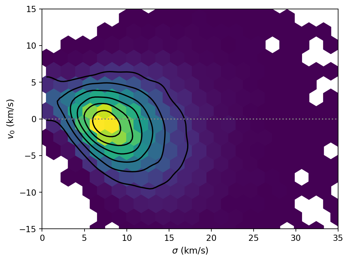
def plot_pair(ax= None ):= az.plot_pair(= inf_data,= FIGSIZE,= ["sigma" , "v0" ],= LABELLER,= ["hexbin" , "kde" ],= {"cmap" : "YlGn" },= TEXTSIZE,= ax,0 , ** INDICATOR_STYLE)0 , 35 )- 15 , 15 )return ax
Figure
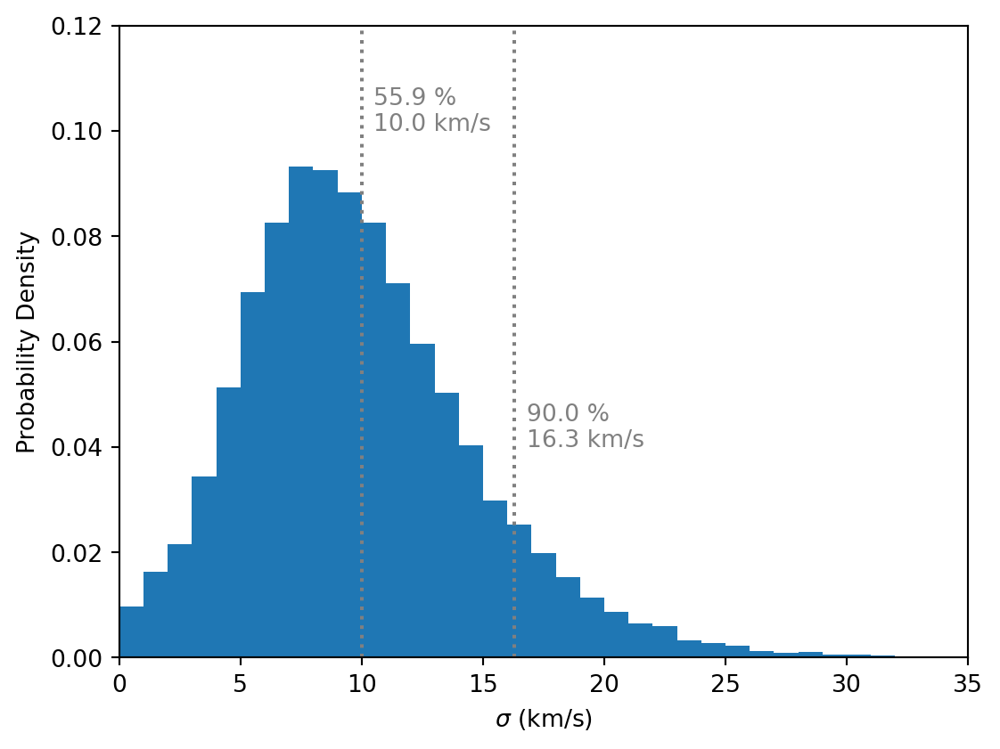
def plot_posterior(ax= None ):if ax is None := plt.subplots(figsize= FIGSIZE)= az.extract(inf_data, var_names= ["sigma" ])= np.arange(0 , 36 , 1 ), density= True )for x, y, p in [10 , 0.1 , scipy.stats.percentileofscore(sigma, 10 )),90 ), 0.04 , 90 ),** INDICATOR_STYLE)+ 0.5 , y + 0.005 , f" { p:.1f} %" , c= INDICATOR_STYLE["c" ])+ 0.5 , y, f" { x:.1f} km/s" , c= INDICATOR_STYLE["c" ])r"$\sigma$ (km/s)" )"Probability Density" )0 , 35 )0 , 0.12 )return ax
Figure 5: The posterior distribution of the velocity dispersion \(\sigma\) .
Figure
def plot_forest(ax= None ):= az.plot_forest(= inf_data,= FIGSIZE,= ["v" ],= "ridgeplot" ,= 0.99 ,= 0.6 ,= 0 ,= True ,= "black" ,= TEXTSIZE,= ax,= _ax[0 ]= 0.825 = np.arange(len (data)) * dy= y[::- 1 ]= data["v" ], y= y, xerr= data["v_err" ], ** MARKER_STYLE)0 , ** INDICATOR_STYLE)= data["name" ])r"$\Delta\,v$ (km/s)" )- 60 , 60 )- dy / 2 , np.max (y) + dy)return ax
Watermark
Python implementation: CPython
Python version       : 3.11.13
IPython version      : 9.7.0

scipy     : 1.16.3
matplotlib: 3.10.7
jax       : 0.8.0
IPython   : 9.7.0
pandas    : 2.3.3
numpy     : 2.3.4
arviz     : 0.22.0
numpyro   : 0.19.0