This notebook is part of a set of examples for teaching Bayesian inference methods and probabilistic programming, using the numpyro library.
Imports
import io

import arviz as az
import jax
import jax.numpy as jnp
import matplotlib.pyplot as plt
import numpy as np
import numpyro
import numpyro.distributions as dist
import numpyro.infer
import pandas as pd

from IPython.display import display
RNG Setup
rng_key = jax.random.PRNGKey(1)
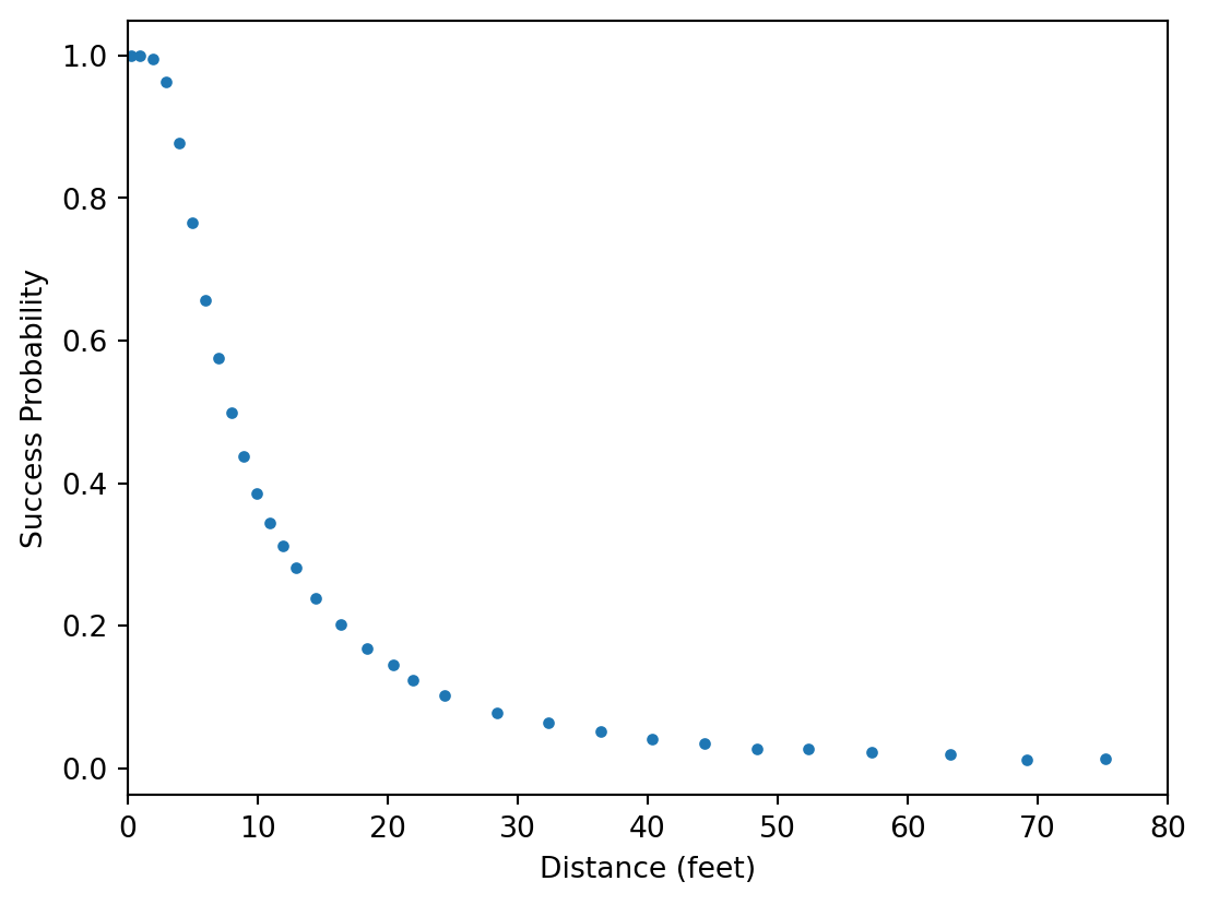
The data consists of the overall number of tries \(\hat{n}\) and successes \(\hat{y}\) for golf putting attempts from certain distances \(\hat{x}\). In this example, we will model the putting success probability \(y/n\) as a function of \(x\).
Data
Data
csv = """
x,n,y
0.28,45198,45183
0.97,183020,182899
1.93,169503,168594
2.92,113094,108953
3.93,73855,64740
4.94,53659,41106
5.94,42991,28205
6.95,37050,21334
7.95,33275,16615
8.95,30836,13503
9.95,28637,11060
10.95,26239,9032
11.95,24636,7687
12.95,22876,6432
14.43,41267,9813
16.43,35712,7196
18.44,31573,5290
20.44,28280,4086
21.95,13238,1642
24.39,46570,4767
28.40,38422,2980
32.39,31641,1996
36.39,25604,1327
40.37,20366,834
44.38,15977,559
48.37,11770,311
52.36,8708,231
57.25,8878,204
63.23,5492,103
69.18,3087,35
75.19,1742,24
"""

data = pd.read_csv(io.StringIO(csv))
Figure
def plot_data(ax=None):
    if ax is None:
        _, ax = plt.subplots(figsize=FIGSIZE)

    ax.plot(data["x"], data["y"] / data["n"], marker=".", ls="none")

    ax.set_xlabel("Distance (feet)")
    ax.set_ylabel("Success Probability")
    ax.set_xlim(0, 80)
    return ax


plot_data()
plt.show()
| 0 |
0.28 |
45198 |
45183 |
| 1 |
0.97 |
183020 |
182899 |
| 2 |
1.93 |
169503 |
168594 |
| 3 |
2.92 |
113094 |
108953 |
| 4 |
3.93 |
73855 |
64740 |
| ... |
... |
... |
... |
| 26 |
52.36 |
8708 |
231 |
| 27 |
57.25 |
8878 |
204 |
| 28 |
63.23 |
5492 |
103 |
| 29 |
69.18 |
3087 |
35 |
| 30 |
75.19 |
1742 |
24 |
31 rows × 3 columns
Model
For a putting attempt to be successful, a golfer needs to hit the ball at the right angle and with the right amount of force.
Let’s assume that the golfer will attempt to hit the ball straight, but that there will be small errors that may cause the angle \(\theta\) at which the ball is hit towards the hole to be non-zero, so that it follows a normal distribution with standard deviation \(\sigma_a\):
\[\theta\sim\text{Normal}(0,\,\sigma_a)\]
The ball will go into the hole if \(\vert\theta\vert<\theta'\), where \(\theta'\) is a threshold angle that depends on the distance \(x\), as well as the radius of the ball \(r=1.68''\), and the radius of the hole \(R=4.25''\):
\[\theta'(x)=\arcsin\left(\frac{R-r}{x}\right)\]
\[p_a(x\vert\sigma_a)=p(\vert\theta\vert<\theta'\vert\sigma_a)=2\Phi\left(\frac{\theta'(x)}{\sigma_a}\right)-1\]
def p_angle(x, sigma, r=1.68 / 2 / 12, R=4.25 / 2 / 12):
    cdf = dist.Normal(0, sigma).cdf
    theta_tol = jnp.rad2deg(jnp.arcsin((R - r) / x))
    return 2.0 * cdf(theta_tol) - 1.0
Let’s also assume that the golfer will attempt to hit the ball with such force that it reaches a distance of \(x_0=1\text{ft}\) beyond the hole, but that there will be small (multiplicative) errors again, so that the target distance \(u\) follows a normal distribution with standard deviation \(\sigma_d\):
\[u\sim\text{Normal}(x+x_0,\,(x+x_0)\,\sigma_d)\]
The ball will go in if \(x<u<x+x'\), that is if it reaches the hole, but does not overshoot by too much. We will assume a maximum tolerance of \(x'=3\text{ft}\).
\[p_d(x\vert\sigma_d)=p(x<u<x+x'\vert\sigma_d)=\Phi\left(\frac{1}{\sigma_d}\frac{x'-x_0}{x+x_0}\right)-\Phi\left(-\frac{1}{\sigma_d}\frac{x_0}{x+x_0}\right)\]
def p_dist(x, sigma, x_0=1, x_tol=3):
    cdf = dist.Normal(0, sigma).cdf
    return cdf((x_tol - x_0) / (x + x_0)) - cdf(-x_0 / (x + x_0))
Finally, the success probability of the putting attempt, taking both effects into account, is:
\[p_t(x\vert\sigma_a,\sigma_d)=p_a(x\vert\sigma_a)\,p_d(x\vert\sigma_d)\]
def p_total(x, sigma_angle, sigma_dist):
    return p_angle(x, sigma_angle) * p_dist(x, sigma_dist)
To balance the weight of the data points at small and large distances, we will not sample the number of successes \(\hat{y}\) directly using a binomial distribution, but by approximation sample the (observed) success probabilities \(\hat{p}_t=\hat{y}/\hat{n}\) from a normal distribution, and allow for some additional variance of \(\hat{p}_t\):
\[\hat{p}_t\sim\text{Normal}\left(p_t,\sqrt{\frac{p_t(1-p_t)}{\hat{n}}+\sigma_e^2}\right)\]
def model(df):
    x_meas = numpyro.param("x_meas", df["x"].values)
    n_meas = numpyro.param("n_meas", df["n"].values)
    y_meas = numpyro.param("y_meas", df["y"].values)

    sigma_angle = numpyro.sample("sigma_angle", dist.HalfNormal(5.0))
    sigma_dist = numpyro.sample("sigma_dist", dist.HalfNormal(5.0))
    sigma_err = numpyro.sample("sigma_err", dist.HalfNormal(5.0))

    with numpyro.plate("data", len(df)):
        p = numpyro.deterministic("p", p_total(x_meas, sigma_angle, sigma_dist))
        p_err = jnp.sqrt(((p * (1 - p)) / n_meas) + sigma_err**2)

        # numpyro.sample("y_obs", dist.Binomial(n_meas, p), obs=y_meas)
        numpyro.sample("p_obs", dist.Normal(p, p_err), obs=y_meas / n_meas)
Figure
numpyro.render_model(
    model=model,
    model_args=(data,),
    render_params=True,
    render_distributions=True,
)
Sampling
sampler = numpyro.infer.MCMC(
    sampler=numpyro.infer.NUTS(model),
    num_warmup=2000,
    num_samples=10000,
    num_chains=4,
    progress_bar=False,
)
rng_key, _rng_key = jax.random.split(rng_key)
sampler.run(_rng_key, data)
inf_data = az.from_numpyro(sampler)
Figure
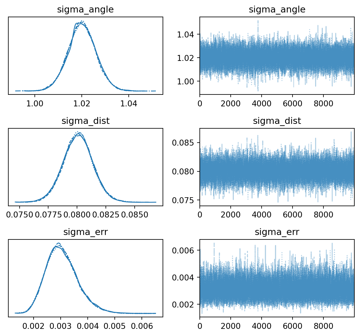
def plot_trace(ax=None):
    return az.plot_trace(
        data=inf_data,
        figsize=(FIGSIZE[0], 3 * 2),
        var_names=["~p"],
        axes=ax,
    )


plot_trace()
plt.tight_layout()
plt.show()
Table
az.summary(inf_data, kind="all", var_names=["~p"])
| sigma_angle |
1.020 |
0.006 |
1.009 |
1.032 |
0.0 |
0.0 |
14589.0 |
17884.0 |
1.0 |
| sigma_dist |
0.080 |
0.001 |
0.078 |
0.083 |
0.0 |
0.0 |
14583.0 |
16386.0 |
1.0 |
| sigma_err |
0.003 |
0.001 |
0.002 |
0.004 |
0.0 |
0.0 |
17658.0 |
19111.0 |
1.0 |
Results
Figure
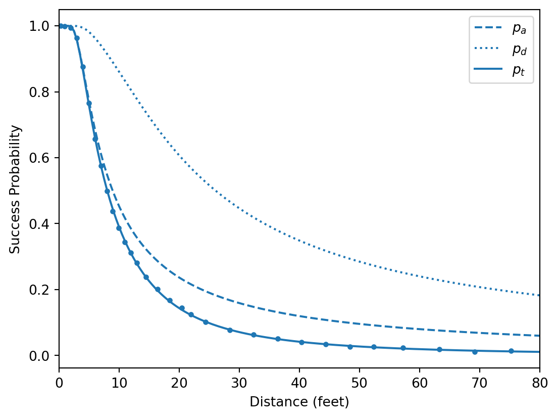
def plot_samples(ax=None):
    ax = plot_data(ax=ax)

    post_mean = az.extract(inf_data).mean("sample")
    sigma_angle = float(post_mean["sigma_angle"])
    sigma_dist = float(post_mean["sigma_dist"])

    x = np.linspace(0, 80, 161)
    ax.plot(x, p_angle(x, sigma_angle), c="C0", ls="dashed", label=r"$p_a$")
    ax.plot(x, p_dist(x, sigma_dist), c="C0", ls="dotted", label=r"$p_d$")
    ax.plot(x, p_total(x, sigma_angle, sigma_dist), c="C0", label=r"$p_t$")

    ax.legend()
    return ax


plot_samples()
plt.show()
Watermark
Python implementation: CPython
Python version       : 3.11.13
IPython version      : 9.7.0

numpy     : 2.3.4
jax       : 0.8.0
pandas    : 2.3.3
IPython   : 9.7.0
matplotlib: 3.10.7
arviz     : 0.22.0
numpyro   : 0.19.0