The Tadpole Case

Binomial Distribution
Real World
Logits

This notebook is part of a set of examples for teaching Bayesian inference methods and probabilistic programming, using the numpyro library.

Imports
import io

import arviz as az
import jax
import matplotlib.pyplot as plt
import numpy as np
import numpyro
import numpyro.distributions as dist
import numpyro.infer
import pandas as pd

from IPython.display import display
from scipy.special import expit
Constants
FIGSIZE = (6.4, 4.8)
TEXTSIZE = 10
RNG Setup
rng_key = jax.random.PRNGKey(1)

The data consists of the initial and final numbers of surviving reed frog tadpoles that were held for some duration in a set of tanks, under similar conditions, except that some were exposed to predators (dragonflies). In this example, we will model the tadpoles’ probability for survival in the different tanks, taking into account the effect of predators, as well as other inter-tank variability.

Data

Data
csv = """
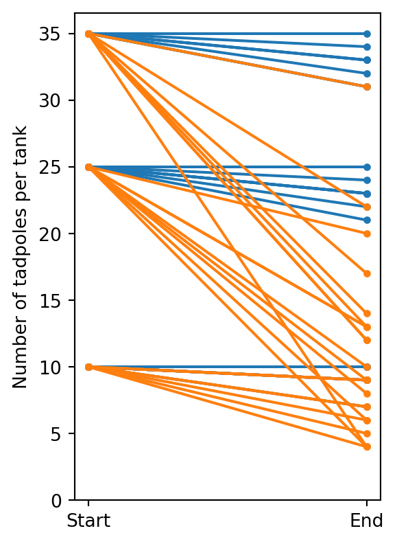
num_start,has_predators,is_large,num_end
10,0,1,9
10,0,1,10
10,0,1,7
10,0,1,10
10,0,0,9
10,0,0,9
10,0,0,10
10,0,0,9
10,1,1,4
10,1,1,9
10,1,1,7
10,1,1,6
10,1,0,7
10,1,0,5
10,1,0,9
10,1,0,9
25,0,1,24
25,0,1,23
25,0,1,22
25,0,1,25
25,0,0,23
25,0,0,23
25,0,0,23
25,0,0,21
25,1,1,6
25,1,1,13
25,1,1,4
25,1,1,9
25,1,0,13
25,1,0,20
25,1,0,8
25,1,0,10
35,0,1,34
35,0,1,33
35,0,1,33
35,0,1,31
35,0,0,31
35,0,0,35
35,0,0,33
35,0,0,32
35,1,1,4
35,1,1,12
35,1,1,13
35,1,1,14
35,1,0,22
35,1,0,12
35,1,0,31
35,1,0,17
"""

data = pd.read_csv(io.StringIO(csv))
data = data.drop(columns=["is_large"])
Figure
def plot_data(ax=None):
    if ax is None:
        _, ax = plt.subplots(figsize=(3, FIGSIZE[1]))

    x = [0, 1]
    for i, d in data.iterrows():
        y = [d["num_start"], d["num_end"]]
        ax.plot(x, y, c="C1" if d["has_predators"] else "C0", marker=".")

    ax.set_xticks(x, labels=["Start", "End"])
    ax.set_ylim(0, None)
    ax.set_ylabel("Number of tadpoles per tank")
    return ax


plot_data()
plt.show()

Figure 1: The number of tadpoles per tank, at the start and end of the experiment. For each tank, line color indicates the presence (orange) or absence (blue) of predators.
num_start has_predators num_end
0 10 0 9
1 10 0 10
2 10 0 7
3 10 0 10
4 10 0 9
... ... ... ...
43 35 1 14
44 35 1 22
45 35 1 12
46 35 1 31
47 35 1 17

48 rows × 3 columns

Model

For each tank \(i\), let’s express the tadpoles’ survival probability as \(p_i=\text{logit}(\alpha_i)\), where the log-odds \(\alpha_i=\alpha_{t,i}+\alpha_p\) have a tank-dependent term \(\alpha_{t,i}\), and a predator-dependent term \(\alpha_p\) that is zero in the absence of predators.

def model(df):
    num_start = numpyro.param("num_start", df["num_start"].values)
    num_end = numpyro.param("num_end", df["num_end"].values)
    has_predators = numpyro.param("has_predators", df["has_predators"].values)

    mean = numpyro.sample("mean", dist.Normal(0, 1.5))
    sigma = numpyro.sample("sigma", dist.Exponential(1))

    alpha_p = numpyro.sample("alpha_p", dist.Normal(0, 0.5))

    with numpyro.plate("tank", len(data)):
        alpha_t = numpyro.sample("alpha_t", dist.Normal(mean, sigma))

        alpha = numpyro.deterministic("alpha", alpha_t + alpha_p * has_predators)
        numpyro.sample("num_obs", dist.Binomial(num_start, logits=alpha), obs=num_end)
Figure
numpyro.render_model(
    model=model,
    model_args=(data,),
    render_params=True,
    render_distributions=True,
)

Figure 2: The model graph.

Sampling

sampler = numpyro.infer.MCMC(
    sampler=numpyro.infer.NUTS(model),
    num_warmup=2000,
    num_samples=10000,
    num_chains=4,
    progress_bar=False,
)
rng_key, _rng_key = jax.random.split(rng_key)
sampler.run(_rng_key, data)
inf_data = az.from_numpyro(sampler)
inf_data.posterior["p"] = expit(inf_data.posterior["alpha"])
Figure
def plot_trace(ax=None):
    return az.plot_trace(
        data=inf_data,
        figsize=(FIGSIZE[0], 4 * 2),
        var_names=["~alpha", "~p"],
        axes=ax,
    )


plot_trace()
plt.tight_layout()
plt.show()

Figure 3: The MCMC trace plot.
Table
az.summary(inf_data, kind="all", var_names=["~alpha_t", "~alpha", "~p"])
mean sd hdi_3% hdi_97% mcse_mean mcse_sd ess_bulk ess_tail r_hat
alpha_p -1.823 0.304 -2.405 -1.262 0.004 0.003 6097.0 9477.0 1.0
mean 2.194 0.230 1.767 2.633 0.002 0.002 9094.0 15609.0 1.0
sigma 0.913 0.168 0.613 1.235 0.002 0.001 11742.0 20416.0 1.0

Results

Figure
def plot_forest(ax=None):
    _ax = az.plot_forest(
        data=inf_data,
        figsize=(FIGSIZE[0], 0.2 * len(data)),
        var_names=["p"],
        combined=True,
        colors="black",
        markersize=10 * 0.75,
        textsize=TEXTSIZE,
        ax=ax,
    )

    ax = _ax[0]
    dy = 0.825
    y = np.arange(len(data)) * dy
    y = y[::-1]

    mask = data["has_predators"].values == 1

    post_mean = az.extract(inf_data).mean("sample")

    p_m = expit(float(post_mean["mean"]) + mask * float(post_mean["alpha_p"]))
    ax.plot(p_m, y, ls="none", marker="|", ms=10, c="black")

    p_t = expit(post_mean["alpha_t"])
    ax.plot(p_t[mask], y[mask], ls="none", marker=".", ms=10, mfc="none", mec="black")

    p_obs = data["num_end"] / data["num_start"]
    ax.plot(p_obs, y, ls="none", marker="D", ms=5, mfc="1", mec="0")

    colors = np.where(mask, "C1", "C0")
    for i, d in data.iterrows():
        y1, y2 = y[i] - dy / 2, y[i] + dy / 2
        ax.fill_between([0, 1], y1, y2, color=colors[i], ec="none", alpha=0.1)

    ax.axhline(np.mean(y[15:17]), c="black", ls="dashed")
    ax.axhline(np.mean(y[31:33]), c="black", ls="dashed")

    ax.set_yticks([])
    ax.set_xlabel(r"$p$")
    ax.set_ylim(-dy / 2, np.max(y) + dy / 2)
    return ax


plot_forest()
plt.show()

Figure 4: The predicted survival probability of tadpoles per tank (filled circles, bars), shown together with the observed values (diamonds). For each tank, the background color indicates the presence (orange) or absence (blue) of predators. The mean survival probability is also shown for both situations (vertical lines), as well as the expected per-tank survival probability in the absence of predators (hollow circles).

Resources

Watermark

Python implementation: CPython
Python version       : 3.11.7
IPython version      : 8.20.0

arviz     : 0.17.0
numpy     : 1.26.3
pandas    : 2.1.4
matplotlib: 3.8.2
numpyro   : 0.13.2
jax       : 0.4.23