The Virus Case

This notebook is part of a set of examples for teaching Bayesian inference methods and probabilistic programming, using the numpyro library.

Imports

import io

import arviz as az
import jax
import jax.numpy as jnp
import matplotlib.pyplot as plt
import numpy as np
import numpyro
import numpyro.distributions as dist
import numpyro.infer
import pandas as pd

from arviz.labels import MapLabeller
from IPython.display import display
from jax.experimental.ode import odeint

Constants

FIGSIZE = (6.4, 4.8)
TEXTSIZE = 10

LABELLER = MapLabeller({"R0": r"$R_0$", "tau": r"$\tau$ (days)"})

RNG Setup

rng_key = jax.random.PRNGKey(1)

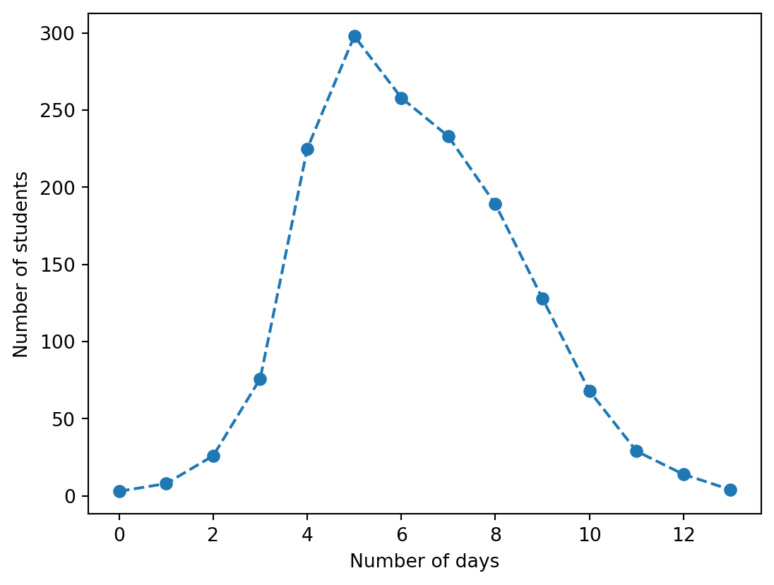
The data consists of the daily number of sick students (listed “in bed”) over the course of an influenza outbreak that occurred at a British boarding school in 1978, a relatively closed community. In this example, we will model this outbreak using a Susceptible-Infected-Resistant (SIR) model.

Data

Data

csv = """
date,in_bed,convalescent
1978-01-22,3,0
1978-01-23,8,0
1978-01-24,26,0
1978-01-25,76,0
1978-01-26,225,9
1978-01-27,298,17
1978-01-28,258,105
1978-01-29,233,162
1978-01-30,189,176
1978-01-31,128,166
1978-02-01,68,150
1978-02-02,29,85
1978-02-03,14,47
1978-02-04,4,20
"""

data = pd.read_csv(io.StringIO(csv), parse_dates=[0])
data["t"] = (data["date"] - data["date"].iloc[0]).dt.days
data = data.drop(columns=["convalescent"])

Figure

def plot_data(plot_kwargs=None, ax=None):
    if ax is None:
        _, ax = plt.subplots(figsize=FIGSIZE)

    plot_kwargs = {"marker": "o", "ls": "dashed", "legend": None, **(plot_kwargs or {})}
    data.plot(x="t", y="in_bed", c="C0", label=r"$\hat{I}$", **plot_kwargs, ax=ax)

    ax.set_xlabel("Number of days")
    ax.set_ylabel("Number of students")
    return ax


plot_data()
plt.show()

Figure 1: The daily number of sick students over the course of the outbreak.

	date	in_bed	t
0	1978-01-22	3	0
1	1978-01-23	8	1
2	1978-01-24	26	2
3	1978-01-25	76	3
4	1978-01-26	225	4
5	1978-01-27	298	5
6	1978-01-28	258	6
7	1978-01-29	233	7
8	1978-01-30	189	8
9	1978-01-31	128	9
10	1978-02-01	68	10
11	1978-02-02	29	11
12	1978-02-03	14	12
13	1978-02-04	4	13

Model

The time evolution of the susceptible population \(S(t)\), the infected (and infectious) population \(I(t)\), and the resistant population \(R(t)\) of students is linked. Let’s assume that when a susceptible student comes into contact with an infected one, the former can become infected for some time, and will become resistant (immune) after recovery. If \(\beta\) is the infection rate, \(\gamma\) the recovery rate, and the total number of students \(N=S+I+R=763\) does not change, then:

\[ \begin{align} \frac{dS}{dt}&=-\beta\,\frac{I}{N}\,S\\ \frac{dI}{dt}&=\beta\,\frac{I}{N}\,S-\gamma\,I\\ \frac{dR}{dt}&=\gamma\,I \end{align} \]

def sir(y, t, theta, n):
    S, I, R = y
    beta, gamma = theta

    dS_dt = -beta * I * S / n
    dI_dt = beta * I * S / n - gamma * I
    dR_dt = gamma * I

    return jnp.array([dS_dt, dI_dt, dR_dt])

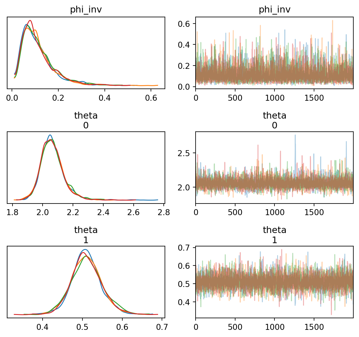
Let’s also assume that the outbreak started with one infected student, so that \(I(0)=1\), \(R(0)=0\), and \(S(0)=N-I(0)\). As the sampling distribution for the number of infected students, we will use the negative binomial distribution, which allows us to take overdispersion of the counts into account (relative to a Poisson distribution), by means of an additional parameter \(\phi\).

def model(df=None, t=None, n=763.0, I0=1.0, R0=0.0, ode_kwargs=None):
    ode_kwargs = {"rtol": 1e-6, "atol": 1e-5, "mxstep": 1000, **(ode_kwargs or {})}

    y0 = numpyro.param("y0", jnp.array([n - I0, I0, R0]))

    if t is None:
        assert df is not None
        _t = numpyro.param("t_meas", df["t"].values.astype(float))
        y_meas = numpyro.param("y_meas", df["in_bed"].values)
    else:
        assert df is None
        _t = numpyro.param("t", t_pred.astype(float))
        y_meas = None

    theta = numpyro.sample(
        "theta",
        dist.TruncatedNormal(
            jnp.array([2.0, 0.4]),
            jnp.array([1.0, 0.5]),
            low=0.0,
        ),
    )

    phi = 1 / numpyro.sample("phi_inv", dist.Exponential(5))

    with numpyro.plate("data", len(_t)):
        y = numpyro.deterministic("y", odeint(sir, y0, _t, theta, n, **ode_kwargs))
        numpyro.sample("y_obs", dist.NegativeBinomial2(y[:, 1], phi), obs=y_meas)

Figure

numpyro.render_model(
    model=model,
    model_args=(data,),
    render_params=True,
    render_distributions=True,
)

Figure 2: The model graph.

Sampling

sampler = numpyro.infer.MCMC(
    sampler=numpyro.infer.NUTS(model),
    num_warmup=1000,
    num_samples=2000,
    num_chains=4,
    progress_bar=False,
)

rng_key, _rng_key = jax.random.split(rng_key)
sampler.run(_rng_key, data)

inf_data = az.from_numpyro(sampler)

beta, gamma = inf_data.posterior["theta"].transpose("theta_dim_0", ...)
inf_data.posterior["R0"] = beta / gamma
inf_data.posterior["tau"] = 1 / gamma

Figure

def plot_trace(ax=None):
    return az.plot_trace(
        data=inf_data,
        figsize=(FIGSIZE[0], 3 * 2),
        var_names=["~y", "~R0", "~tau"],
        compact=False,
        axes=ax,
    )


plot_trace()
plt.tight_layout()
plt.show()

Figure 3: The MCMC trace plot.

Table

az.summary(inf_data, kind="all", var_names=["~y"])

	mean	sd	hdi_3%	hdi_97%	mcse_mean	mcse_sd	ess_bulk	ess_tail	r_hat
phi_inv	0.113	0.072	0.018	0.245	0.001	0.001	3918.0	4201.0	1.0
theta[0]	2.064	0.078	1.927	2.211	0.001	0.001	4268.0	3364.0	1.0
theta[1]	0.511	0.039	0.440	0.588	0.001	0.000	4350.0	4068.0	1.0
R0	4.069	0.389	3.338	4.762	0.007	0.005	3937.0	3409.0	1.0
tau	1.969	0.151	1.679	2.246	0.002	0.002	4350.0	4068.0	1.0

Results

predictive = numpyro.infer.Predictive(model, sampler.get_samples())

t_pred = np.linspace(0, 14, 50)

rng_key, _rng_key = jax.random.split(rng_key)
pred_data = az.from_numpyro(posterior_predictive=predictive(_rng_key, t=t_pred))

Figure

def plot_pred(ax=None):
    ax = plot_data(plot_kwargs={"ls": "None"}, ax=ax)

    pred_mean = az.extract(pred_data, group="posterior_predictive").mean("sample")
    pred_hdi = az.hdi(pred_data, group="posterior_predictive")

    ax.plot(t_pred, pred_mean["y"].sel(y_dim_1=0), c="C0", ls="dashed", label=r"$S$")
    ax.plot(t_pred, pred_mean["y"].sel(y_dim_1=2), c="C0", ls="dotted", label=r"$R$")

    ax.plot(t_pred, pred_mean["y_obs"], c="C0", label=r"$I$")

    az.plot_hdi(x=t_pred, hdi_data=pred_hdi["y_obs"], color="C0", smooth=False, ax=ax)

    ax.legend()
    return ax


plot_pred()
plt.show()

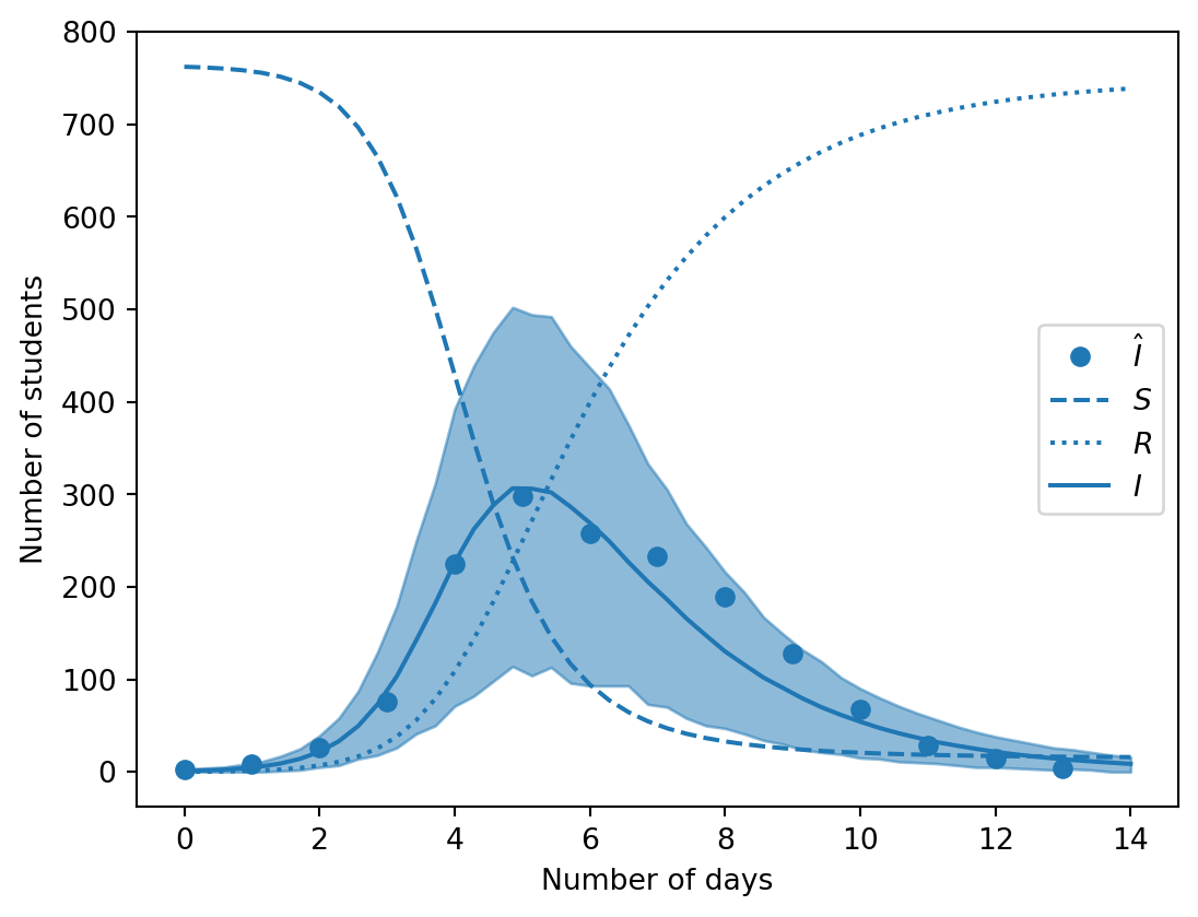
Figure 4: The predicted number of infected students (\(I\)), as well as the number of susceptible students (\(S\)) and resistant students (\(R\)), over the course of the outbreak, shown together with the observed counts (\(\hat{I}\)).

Figure

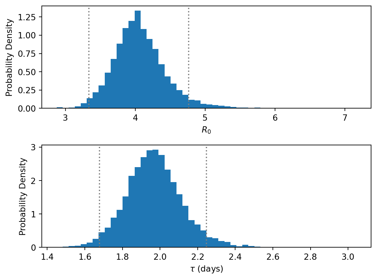
def plot_posterior(ax=None):
    if ax is None:
        _, ax = plt.subplots(2, 1, figsize=FIGSIZE)

    post = az.extract(inf_data, var_names=["R0", "tau"])
    post_hdi = az.hdi(inf_data, var_names=["R0", "tau"])

    for i, (name, values) in enumerate(post.items()):
        ax[i].hist(values, bins=50, density=True)

        for value in post_hdi[name]:
            ax[i].axvline(x=value, c="gray", ls="dotted")

        ax[i].set_xlabel(LABELLER.var_name_to_str(name))
        ax[i].set_ylabel("Probability Density")

    return ax


plot_posterior()
plt.tight_layout()
plt.show()

Figure 5: The posterior distributions of the basic reproduction number \(R_0=\beta/\gamma\) and the recovery time \(\tau=1/\gamma\).

Resources

• Bayesian workflow for disease transmission modeling in Stan (Grinsztajn+ 2020, Stan Case Studies)

Watermark

Python implementation: CPython
Python version       : 3.11.7
IPython version      : 8.20.0

numpy     : 1.26.3
numpyro   : 0.13.2
jax       : 0.4.23
matplotlib: 3.8.2
pandas    : 2.1.4
arviz     : 0.17.0