This notebook is part of a set of examples for teaching Bayesian inference methods and probabilistic programming, using the numpyro library.
Imports
import io

import arviz as az
import jax
import jax.numpy as jnp
import matplotlib.pyplot as plt
import numpy as np
import numpyro
import numpyro.distributions as dist
import numpyro.infer
import pandas as pd

from IPython.display import display
from jax.experimental.ode import odeint
Constants
FIGSIZE = (6.4, 4.8)
TEXTSIZE = 10
RNG Setup
rng_key = jax.random.PRNGKey(1)
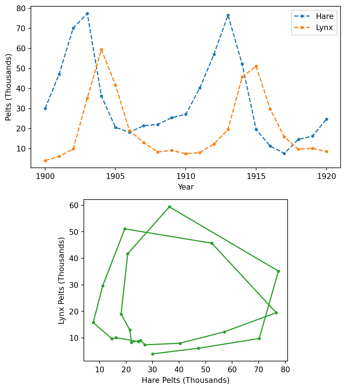
The data consists of the number of pelts of the Canadian lynx and the snowshoe hare collected annually between 1900 and 1920. These two species are in a predator-prey relationship, and their population sizes oscillate. In this example, we will use the Lotka-Volterra equations to model these oscillations, taking the number of collected pelts as a proxy for population size.
Data
Data
csv = """
year,lynx,hare
1900,4.0,30.0
1901,6.1,47.2
1902,9.8,70.2
1903,35.2,77.4
1904,59.4,36.3
1905,41.7,20.6
1906,19.0,18.1
1907,13.0,21.4
1908,8.3,22.0
1909,9.1,25.4
1910,7.4,27.1
1911,8.0,40.3
1912,12.3,57.0
1913,19.5,76.6
1914,45.7,52.3
1915,51.1,19.5
1916,29.7,11.2
1917,15.8,7.6
1918,9.7,14.6
1919,10.1,16.2
1920,8.6,24.7
"""

data = pd.read_csv(io.StringIO(csv))
data["t"] = data["year"] - data["year"].iloc[0]
Figure
def plot_data_timeline(plot_kwargs=None, ax=None):
    if ax is None:
        _, ax = plt.subplots(figsize=FIGSIZE)

    plot_kwargs = {"marker": ".", "ls": "dashed"} | (plot_kwargs or {})
    data.plot(x="year", y="hare", c="C0", label="Hare", **plot_kwargs, ax=ax)
    data.plot(x="year", y="lynx", c="C1", label="Lynx", **plot_kwargs, ax=ax)

    ax.set_xticks(np.arange(1900, 1921, 5))
    ax.set_xlabel("Year")
    ax.set_ylabel("Pelts (Thousands)")
    return ax


def plot_data_correlation(ax=None):
    if ax is None:
        _, ax = plt.subplots(figsize=FIGSIZE)

    data.plot(x="hare", y="lynx", c="C2", marker=".", legend=None, ax=ax)

    ax.set_xlabel("Hare Pelts (Thousands)")
    ax.set_ylabel("Lynx Pelts (Thousands)")
    ax.set_aspect("equal")
    return ax


def plot_data(ax=None):
    if ax is None:
        _, ax = plt.subplots(2, 1, figsize=(FIGSIZE[0], 1.5 * FIGSIZE[1]))

    plot_data_timeline(ax=ax[0])
    plot_data_correlation(ax=ax[1])

    return ax


plot_data()
plt.tight_layout()
plt.show()
| 0 |
1900 |
4.0 |
30.0 |
0 |
| 1 |
1901 |
6.1 |
47.2 |
1 |
| 2 |
1902 |
9.8 |
70.2 |
2 |
| 3 |
1903 |
35.2 |
77.4 |
3 |
| 4 |
1904 |
59.4 |
36.3 |
4 |
| 5 |
1905 |
41.7 |
20.6 |
5 |
| 6 |
1906 |
19.0 |
18.1 |
6 |
| 7 |
1907 |
13.0 |
21.4 |
7 |
| 8 |
1908 |
8.3 |
22.0 |
8 |
| 9 |
1909 |
9.1 |
25.4 |
9 |
| 10 |
1910 |
7.4 |
27.1 |
10 |
| 11 |
1911 |
8.0 |
40.3 |
11 |
| 12 |
1912 |
12.3 |
57.0 |
12 |
| 13 |
1913 |
19.5 |
76.6 |
13 |
| 14 |
1914 |
45.7 |
52.3 |
14 |
| 15 |
1915 |
51.1 |
19.5 |
15 |
| 16 |
1916 |
29.7 |
11.2 |
16 |
| 17 |
1917 |
15.8 |
7.6 |
17 |
| 18 |
1918 |
9.7 |
14.6 |
18 |
| 19 |
1919 |
10.1 |
16.2 |
19 |
| 20 |
1920 |
8.6 |
24.7 |
20 |
Model
If \(u(t)\) is the population size of the prey species (hare) at time \(t\) and \(v(t)\) the population size of the predator species (lynx), the time evolution of \(\boldsymbol{y}_t=[u(t),v(t)]\), starting from some initial populations \(\boldsymbol{y}_0\), can be described by a pair of differential equations depending on four non-negative parameters \(\boldsymbol{\theta}=[\alpha,\beta,\gamma,\delta]\), known as the Lotka-Volterra equations:
\[\frac{d\boldsymbol{y}}{dt}=\left[\frac{du}{dt},\frac{dv}{dt}\right]=\left[(\alpha-\beta\,v)\,u,(-\gamma+\delta\,u)\,v\right]\]
def dy_dt(y, t, theta):
    du_dt = (theta[..., 0] - theta[..., 1] * y[1]) * y[0]
    dv_dt = (-theta[..., 2] + theta[..., 3] * y[0]) * y[1]
    return jnp.stack([du_dt, dv_dt])
Instead of modeling the population sizes \(\boldsymbol{y}_t\) directly, it is convenient to model the log-transformed values \(\log(\boldsymbol{y}_t)\), which are not contrained to be positive. Let’s also assume that there will be some (multiplicative) errors in measuring \(\boldsymbol{y}_t\), so that the observed population sizes \(\hat{\boldsymbol{y}}_t\) are expected to follow a log-normal distribution with standard deviation \(\boldsymbol{\sigma}\):
\[\log(\hat{\boldsymbol{y}}_t)\sim\text{Normal}(\log(\boldsymbol{z}_t),\boldsymbol{\sigma})\]
def model(df=None, t=None, ode_kwargs=None):
    ode_kwargs = {"rtol": 1e-6, "atol": 1e-3, "mxstep": 1000} | (ode_kwargs or {})

    if t is None:
        assert df is not None
        _t = numpyro.param("t_meas", df["t"].values.astype(float))
        y_meas = numpyro.param("y_meas", df[["hare", "lynx"]].values)
    else:
        assert df is None
        _t = numpyro.param("t", t.astype(float))
        y_meas = None

    theta = numpyro.sample(
        "theta",
        dist.TruncatedNormal(
            jnp.array([1.0, 0.05, 1.0, 0.05]),
            jnp.array([0.5, 0.05, 0.5, 0.05]),
            low=0.0,
        ),
    )

    with numpyro.plate("species", 2):
        y0 = numpyro.sample("y0", dist.LogNormal(jnp.log(10), 1).expand([2]))
        sigma = numpyro.sample("sigma", dist.LogNormal(-1, 1).expand([2]))

        with numpyro.plate("data", len(_t)):
            y = numpyro.deterministic("y", odeint(dy_dt, y0, _t, theta, **ode_kwargs))
            numpyro.sample("y_obs", dist.LogNormal(jnp.log(y), sigma), obs=y_meas)
Figure
numpyro.render_model(
    model=model,
    model_args=(data,),
    render_params=True,
    render_distributions=True,
)
Sampling
sampler = numpyro.infer.MCMC(
    sampler=numpyro.infer.NUTS(
        model,
        init_strategy=numpyro.infer.init_to_median(num_samples=1000),
    ),
    num_warmup=1000,
    num_samples=2000,
    num_chains=4,
    progress_bar=False,
)
rng_key, _rng_key = jax.random.split(rng_key)
sampler.run(_rng_key, data)
inf_data = az.from_numpyro(sampler)
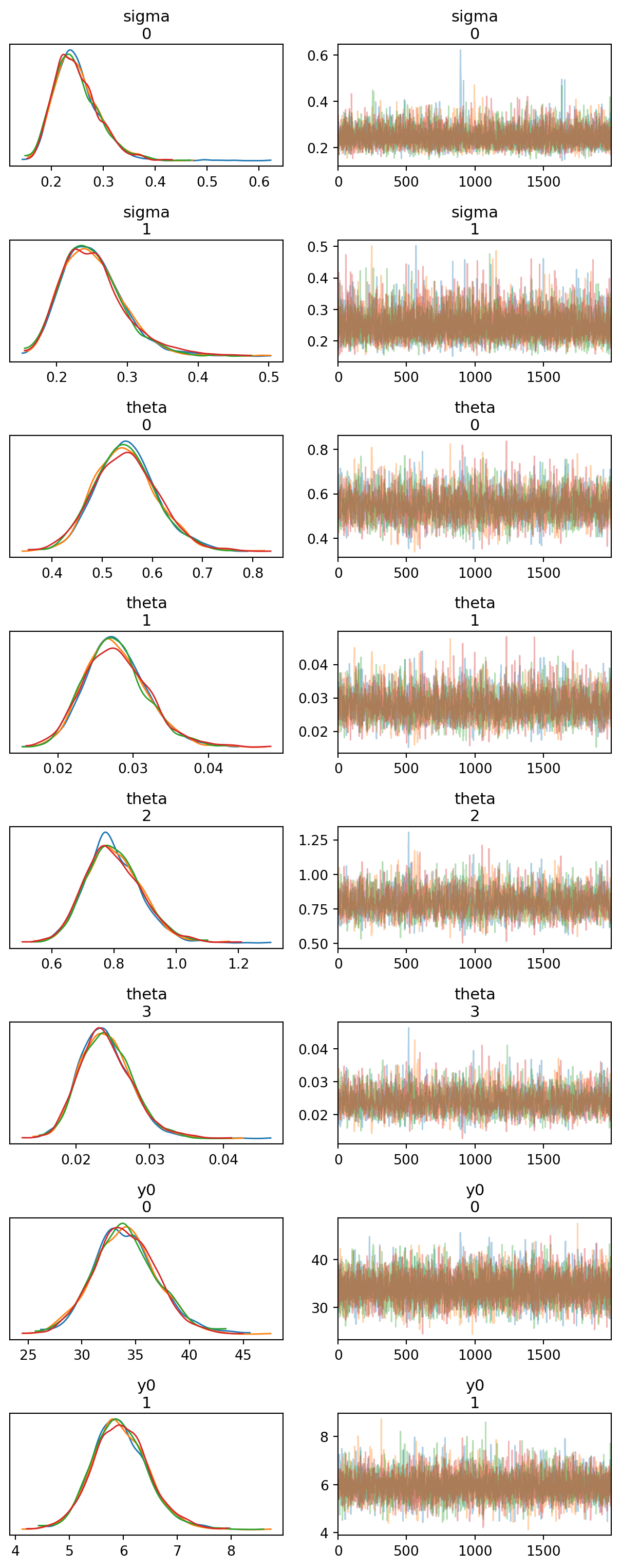
Figure
def plot_trace(ax=None):
    return az.plot_trace(
        data=inf_data,
        figsize=(FIGSIZE[0], 8 * 2),
        var_names=["~y"],
        compact=False,
        axes=ax,
    )


plot_trace()
plt.tight_layout()
plt.show()
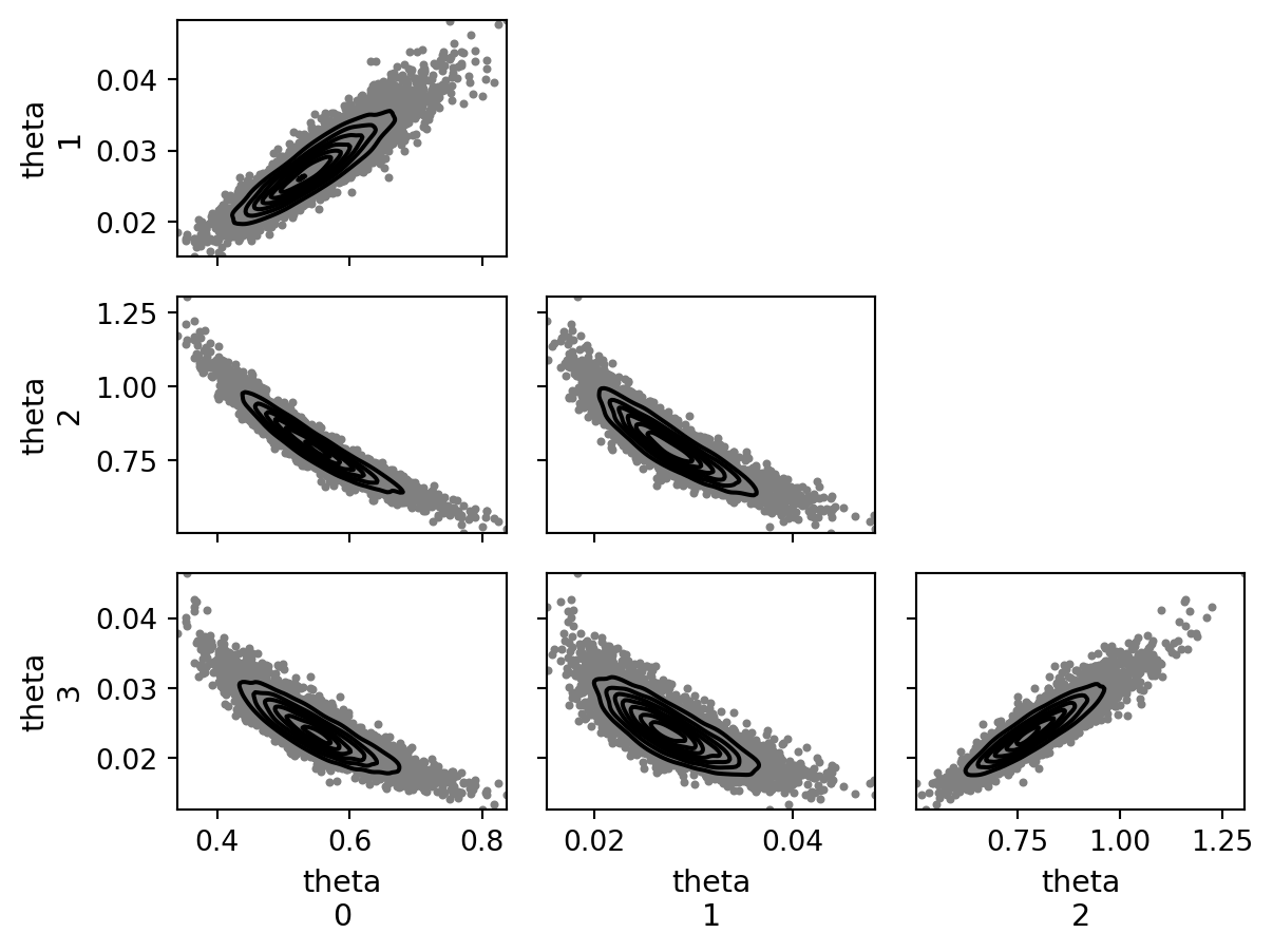
Figure
def plot_pair(ax=None):
    return az.plot_pair(
        data=inf_data,
        figsize=FIGSIZE,
        var_names=["theta"],
        kind=["hexbin", "kde"],
        hexbin_kwargs={"cmap": "YlGn"},
        textsize=TEXTSIZE,
        ax=ax,
    )


plot_pair()
plt.tight_layout()
plt.show()
Table
az.summary(inf_data, kind="all", var_names=["~y"])
| sigma[0] |
0.248 |
0.044 |
0.173 |
0.330 |
0.001 |
0.001 |
5700.0 |
4676.0 |
1.0 |
| sigma[1] |
0.252 |
0.045 |
0.176 |
0.336 |
0.001 |
0.001 |
5403.0 |
5211.0 |
1.0 |
| theta[0] |
0.549 |
0.063 |
0.431 |
0.665 |
0.001 |
0.001 |
2063.0 |
3130.0 |
1.0 |
| theta[1] |
0.028 |
0.004 |
0.020 |
0.036 |
0.000 |
0.000 |
2248.0 |
3196.0 |
1.0 |
| theta[2] |
0.796 |
0.088 |
0.629 |
0.954 |
0.002 |
0.001 |
2035.0 |
3071.0 |
1.0 |
| theta[3] |
0.024 |
0.003 |
0.017 |
0.030 |
0.000 |
0.000 |
2129.0 |
3210.0 |
1.0 |
| y0[0] |
34.089 |
2.901 |
28.518 |
39.425 |
0.040 |
0.039 |
5198.0 |
4513.0 |
1.0 |
| y0[1] |
5.949 |
0.520 |
5.010 |
6.960 |
0.008 |
0.007 |
4347.0 |
4770.0 |
1.0 |
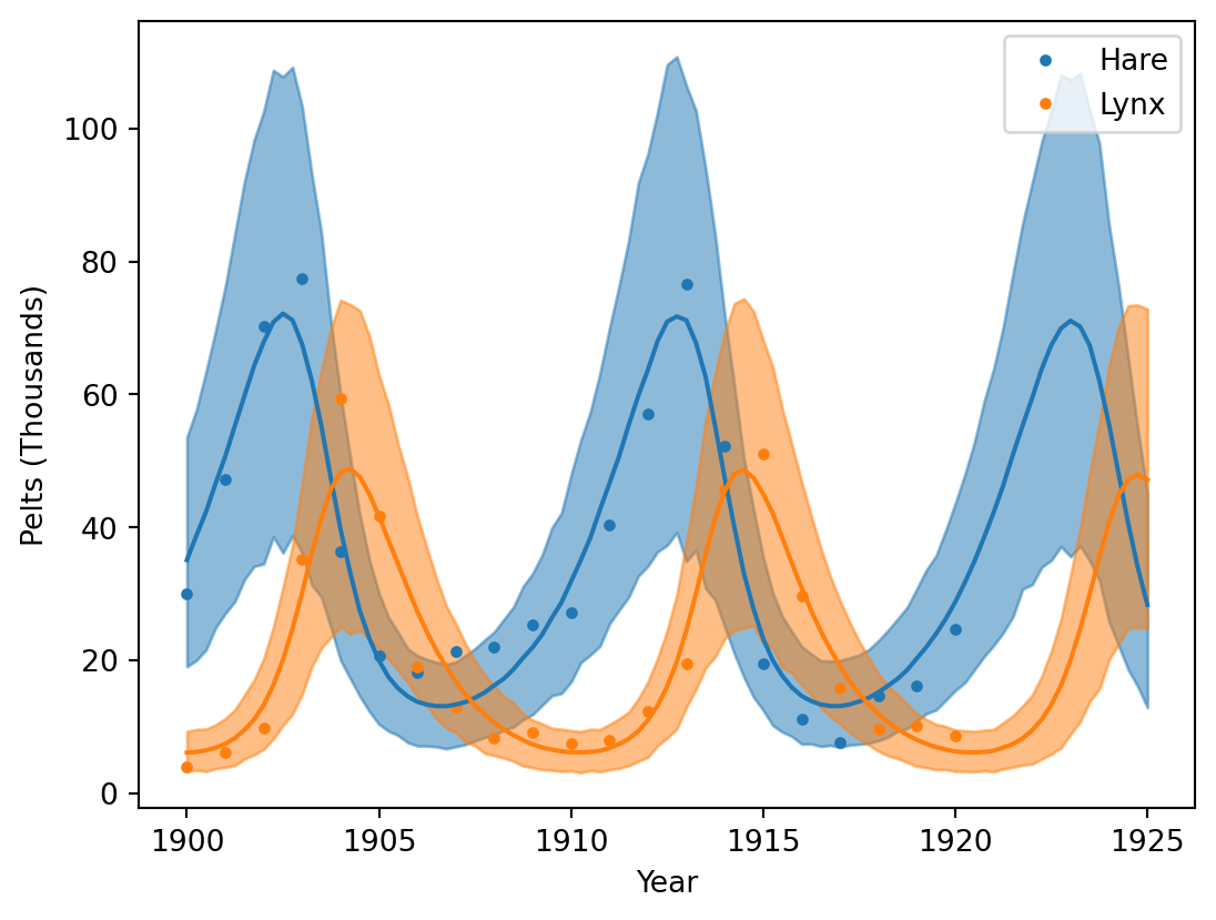
Results
predictive = numpyro.infer.Predictive(model, sampler.get_samples())

t_pred = np.linspace(0, 25, 101)

rng_key, _rng_key = jax.random.split(rng_key)
pred_data = az.from_numpyro(posterior_predictive=predictive(_rng_key, t=t_pred))
Figure
def plot_pred(ax=None):
    ax = plot_data_timeline(plot_kwargs={"ls": "None"}, ax=ax)

    pred_mean = az.extract(pred_data, group="posterior_predictive").mean("sample")
    pred_hdi = az.hdi(pred_data, group="posterior_predictive")

    x = t_pred + data["year"].iloc[0]
    for i in range(2):
        y = pred_mean["y_obs"].sel(y_obs_dim_1=i)
        ax.plot(x, y, c=f"C{i}")

        y = pred_hdi["y_obs"].sel(y_obs_dim_1=i)
        az.plot_hdi(x=x, hdi_data=y, color=f"C{i}", smooth=False, ax=ax)

    ax.set_xticks(np.arange(1900, 1926, 5))
    return ax


plot_pred()
plt.show()
Watermark
Python implementation: CPython
Python version       : 3.11.13
IPython version      : 9.7.0

numpy     : 2.3.4
jax       : 0.8.0
pandas    : 2.3.3
IPython   : 9.7.0
numpyro   : 0.19.0
matplotlib: 3.10.7
arviz     : 0.22.0